CASE · 2026CASE · 2026
Teaching a model to redraw lung tumors, then reusing what it learned
A 3D variational autoencoder learned lung lesion features from CT scans without outcome labels, and those features held up against radiomics for predicting clinical outcomes.
Large language models got good partly because there was an enormous amount of text to learn from, and the text itself was the training signal: predict the next word, and no human has to label anything. Medical imaging does not work like that yet. Hospitals have plenty of scans. What is scarce is labels: which patients had a mutation, whose cancer had reached the lymph nodes, who responded to treatment. Each of those answers costs a pathologist, a genetic test, or years of follow-up.
This project tried to learn something useful about a lung lesion from the image alone, before deciding what we want to predict from it, and then reuse that learning for several different questions.
Two existing ways to turn a scan into numbers
To predict anything from a CT (computed tomography) scan, you first need to turn the picture into numbers a model can work with. There were two common ways to do that.
The first is radiomics. Experts define a long list of measurements in advance (shape, size, brightness statistics, texture patterns) and software computes them from the lesion, usually using a mask that traces its exact boundary. The tool we compared against, PyRadiomics, produces more than 1,600 of these features. They are well understood, but they are fixed: the list does not adapt to the question you are asking.
The second is to train a convolutional neural network (CNN, a model that learns its own image filters) directly on the outcome you care about. That adapts to the question, but it relies on labeled examples. In our comparison, a separate CNN was trained for each question, so a new question meant new labels and a new model.
The idea: learn by redrawing
We used a variational autoencoder, or VAE. It has two halves. The encoder looks at a small 3D block of CT around a lesion and squeezes it down to a short list of numbers. The decoder takes that list and tries to redraw the original block. The model is scored on how close the redrawing is to the original.
The trick is the squeeze. The block has 32 x 32 x 32 voxels (3D pixels), about 3 cm on a side after resampling every scan to 1 mm spacing, so roughly 33,000 values. The encoder has to describe it with 1,024 numbers, plus a matching 1,024 that describe its uncertainty about each one. To redraw well through that bottleneck, the model has to keep enough about the lesion to rebuild it. No one tells it what to keep, and whether what it keeps is clinically useful has to be tested separately. Nothing in this training step uses an outcome label.
The “variational” part means the encoder outputs a mean and a standard deviation for each number (a bell-shaped Gaussian distribution) rather than a single value, and a penalty weighted by a factor called beta pulls those distributions toward a standard Gaussian (hence “beta-VAE”). Our beta was very small (0.00001), so the model was pushed mainly to redraw accurately.
For prediction we set the decoder aside, ran each lesion through the encoder, and handed both sets of 1,024 numbers (the means and the spreads, 2,048 features in all) to XGBoost, a standard tree-based classifier, to predict each clinical outcome.
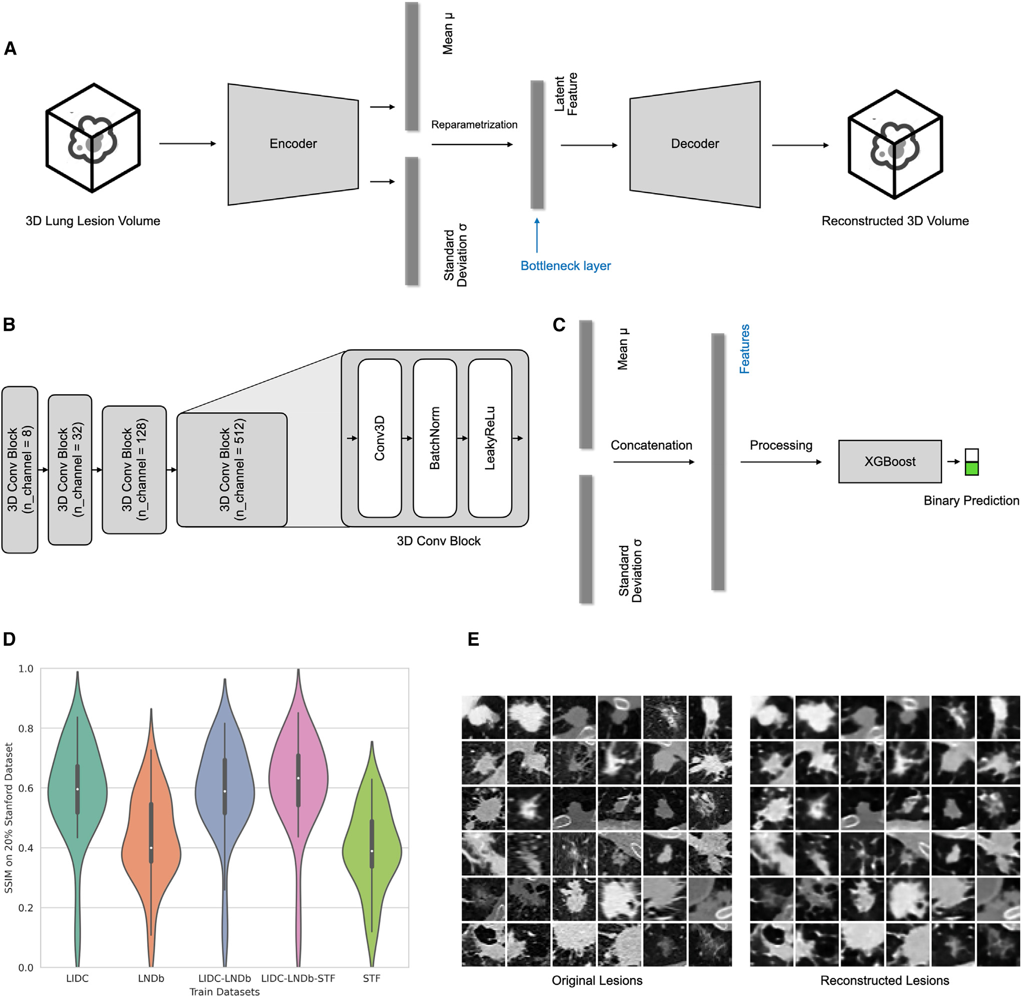 The pipeline: (A) encoder, bottleneck and decoder; (B) the encoder’s four 3D convolution blocks; (C) the learned numbers feeding an XGBoost classifier; (D) reconstruction quality on Stanford test lesions by training data; (E) original lesions next to their reconstructions. Figure 1, Li et al., Cell Reports Methods 2024, CC BY-NC-ND.
The data
We trained on lesions from three sources: two public datasets, LIDC-IDRI (US) and LNDb (Portugal), which together contain thousands of annotated lung nodules, both benign and malignant, and a Stanford radiogenomics cohort of 143 patients with non-small cell lung cancer. Only the Stanford cohort has the clinical and genetic outcomes we wanted to predict, so it is where the downstream tests happened.
One honest caveat about “no labels”: the block is cut around each lesion’s center, and that center comes from an annotation. Marking a center point is much cheaper than tracing a full boundary, but it is still some human input. What the model never sees during this step is the outcome.
How well does it redraw
We measured reconstruction with SSIM, a score that tops out at 1 for how similar two images look in structure, where 1 means identical. On held-out Stanford lesions the model trained on all three datasets reached an SSIM of 0.774, with a peak signal-to-noise ratio of 26.1 and a mean squared error of 0.0008 (two more ways of measuring how far the redraw is from the original). You can see in panel E above that the reconstructions keep each lesion’s overall shape and position but come out smoother than the originals.
The more useful finding was in panel D. Models trained on a single dataset did worst, and the model trained on all three did best. Mixing scans from different hospitals and scanners helped, which matters if you imagine this kind of model improving as more institutions contribute images.
What ended up in the 1,024 numbers
A list of 1,024 numbers is hard to look at, so we used UMAP, a method that squashes high-dimensional data down to two dimensions while trying to keep nearby points nearby. When we sized each lesion’s dot by its volume, small and large lesions sat in different regions of the map, and the correlation between the map position and lesion size was significant (p < 0.001, which says the association is unlikely to be chance, not how strong it is or how well it predicts). Size is the obvious thing to pick up, but it confirms the bottleneck kept something real.
Turning a dial on size
Because the VAE also has a decoder, we can do something radiomics and a supervised CNN cannot: change the numbers and see what picture comes out.
We took the average encoding of the largest Stanford lesions and the average encoding of the smallest, and subtracted one from the other. That difference is a direction in the space of encodings that roughly means “bigger”. Adding it to the encodings of a random batch of 36 Stanford lesions and decoding gave enlarged lesions. Subtracting it gave shrunken ones. When we measured the volumes of the decoded lesions, shrunk ones were smaller and enlarged ones larger than the originals, as intended.
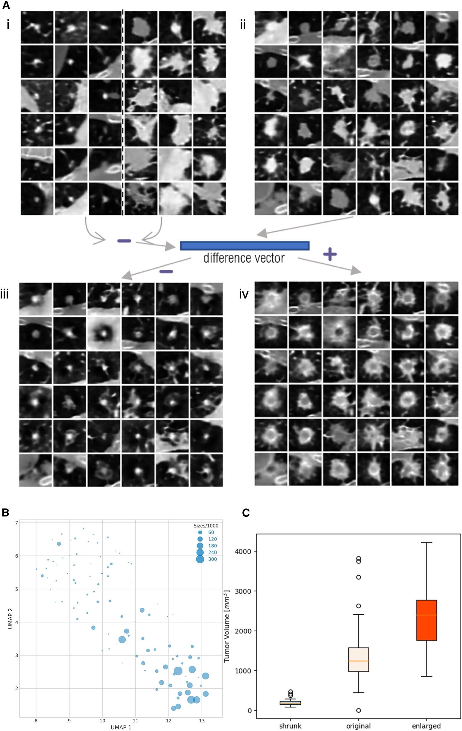 (A) Small and large reference lesions define a size direction, which is subtracted from or added to other lesions; (B) the 2D UMAP map with dot size showing lesion volume; (C) measured volumes of shrunk, original and enlarged lesions. Figure 2, Li et al., Cell Reports Methods 2024, CC BY-NC-ND.
This is what I find most interesting about the project. The decoder gives a two-way bridge between the image and the numbers. If a direction in the numbers seems to matter for a prediction, you can decode along it and look at what changes in the picture. That is a concrete way to explain what a feature stands for, and explanations like that may help clinicians trust a model, though we did not test that.
The limits are just as clear. These are generated images, not a forecast of how a real patient’s tumor will grow. The enlarged lesions developed a hollow look, and the shrunken ones became rounder and more uniform. Push the direction too far and the shapes distort (the paper’s supplementary Figures S3 and S4 show this). And size is the only property we demonstrated; other directions, like texture or margin shape, are untested.
Reusing the features for prediction
The real test of a reusable representation is whether it helps with questions it was never trained on. On the Stanford cohort we framed six clinical questions as yes or no predictions, including KRAS mutation status (a gene whose mutations affect treatment choices), EGFR mutation status, lymphovascular invasion (cancer entering blood or lymph vessels), pathological T stage (tumor size and local extent, T1 versus higher), pathological N stage (whether the cancer has spread to lymph nodes, N0 versus higher), and overall AJCC stage (the combined stage, I versus higher). For each one we compared four feature sets: radiomics, a CNN trained end to end on that question, the VAE features, and radiomics and VAE features combined. Performance was measured with F1, a 0 to 1 score that balances catching the positive cases against raising false alarms, across tenfold cross-validation (split the data into ten parts, test on each part in turn).
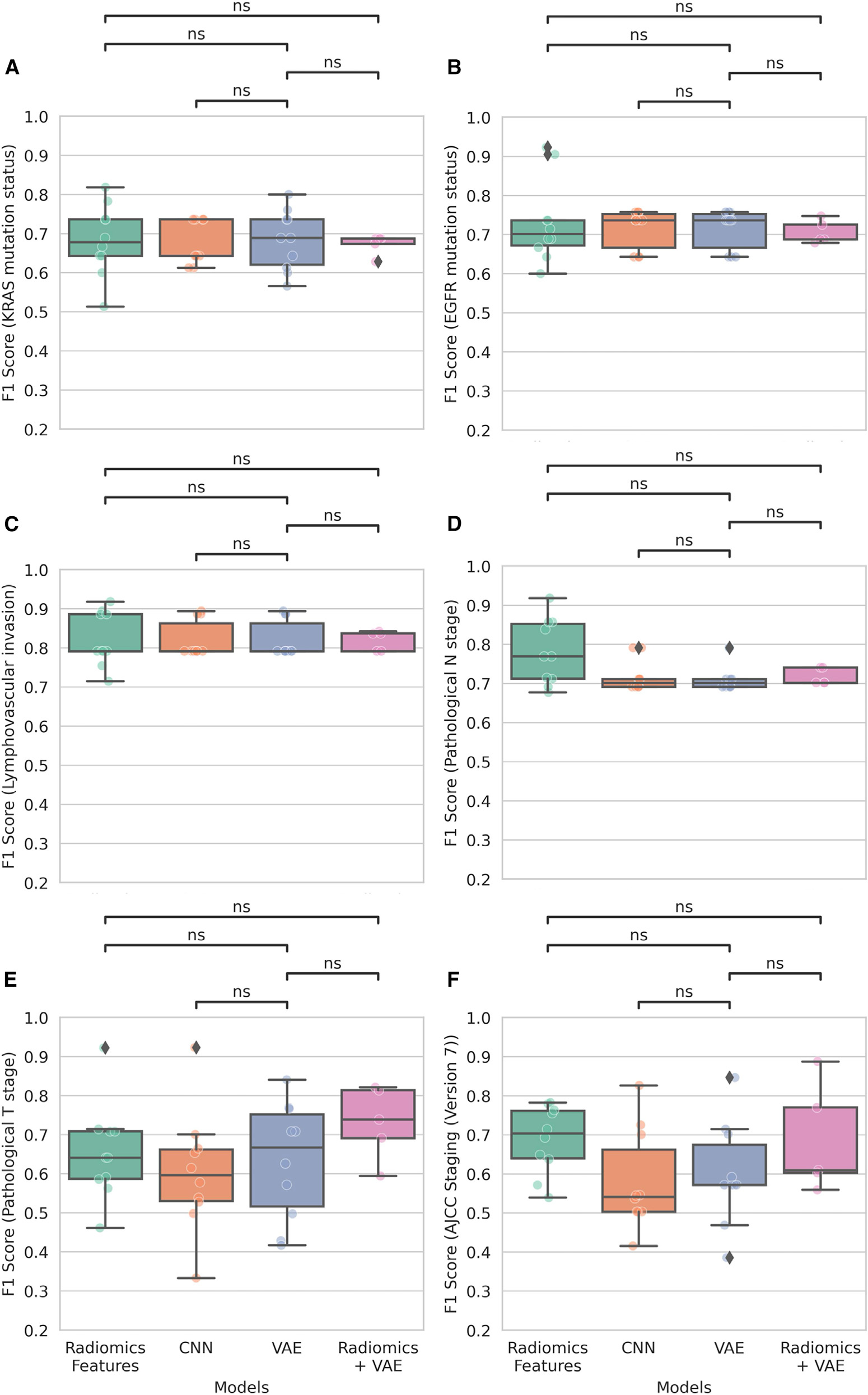 F1 scores of radiomics, a supervised CNN, VAE features, and radiomics plus VAE features on six clinical endpoints in the Stanford cohort; “ns” marks differences that were not statistically significant. Figure 3, Li et al., Cell Reports Methods 2024, CC BY-NC-ND.
Across all six endpoints, none of the differences between the VAE and the other approaches reached statistical significance. For KRAS, the VAE’s scores look much like radiomics and the CNN. For N stage, the radiomics scores sit visibly higher in the plot, even though the test did not call the difference significant. The fair summary is that features learned only by redrawing performed in the same range as hand-designed features that use a detailed lesion boundary, and as a CNN trained directly on each label. That is the result I care about: reconstruction alone produced features useful for later tasks.
The comparison also says something about radiomics and lesion masks: they carry real information, and the VAE did not beat them. Combining the two feature sets did not give a significant improvement either.
What this did not show
It did not show the VAE is better than radiomics, or statistically equivalent to it. “No significant difference” on a cohort of 143 patients is a weak claim in both directions.
It did not remove the need for labels. Finding the lesions still used annotations, and each downstream predictor still needed outcome labels to train. What changed is that the expensive representation-learning step did not.
It is not a clean test on an untouched outside hospital. The Stanford data was part of the combined training set for the VAE, and model selection used a held-out portion of it.
And the size manipulation is a demonstration of what the encoding contains, not a model of tumor growth.
Where this fits
I think about my research through three questions: what data we use, how we train, and how we evaluate. This project is the training one. Medical labels take expert time, so we tried to learn from the images themselves and reuse what we learned for several tasks. The post on COVID-19 CT triage is about the data question, combining a scan with the rest of what is known about a patient. The post on the chest X-ray benchmark is about evaluation: a model that looks good on held-out data can still change when the hospital, the patients, or the task changes, and choosing how to measure that matters as much as the model.
I presented the three projects together in my OpenRefinery talk, “AI for Biomedicine”, in September 2026. The recording is here: https://www.youtube.com/watch?v=Kz_LV64xKjE.
The paper is open access: Li Y., Sadée C.Y., Carrillo-Perez F., Selby H.M., Thieme A.H., Gevaert O. “A 3D lung lesion variational autoencoder.” Cell Reports Methods 4(2):100695, 2024. https://doi.org/10.1016/j.crmeth.2024.100695. The code is at https://github.com/gevaertlab/Variational-Auto-Encoder.