NOTE · 2020笔记 · 2020

Probabilistic Interpretation of Sum of Square Loss Function

One way to interpret the form of "square" in square loss.

2020·04·14 2 MIN2 分钟 #MACHINE-LEARNING#LOSS-FUNCTION#PROBABILITY

Square Loss Function (in Linear Regression)

For linear regression, the way that we used to find the optimal parameters \overrightarrow \theta is called gradient descent, which we seek for \overrightarrow \theta that minimize the loss function:

\mathcal{J}(\theta) = \frac{1}{2} \sum_{i=1}^{n}(y^{(i)} - \theta^T x^{(i)})^2(1)

That is:

\hat \theta = \underset{\theta}{\mathrm{argmin}}[\frac{1}{2} \sum_{i=1}^{n}(y^{(i)} - \theta^T x^{(i)})^2](2)

Interpret the Loss Function as MLE

In linear regression, we assume the model to be:

\overrightarrow y = \theta^T x^{(i)} + \epsilon^{(i)}(3)

where \epsilon is called the error term which conposes of unmodelled factors and random noise. And under general assumption, \epsilon^{(i)}s are gaussian random variables that are independent from each other

\epsilon \in \text{iid }N(0,\sigma^2)(4)

Geometrically, this is the whole story of the square in “square loss”: the line \theta^Tx is not the data, it is the mean of the data, and every observation is drawn from a bell hanging off that line.

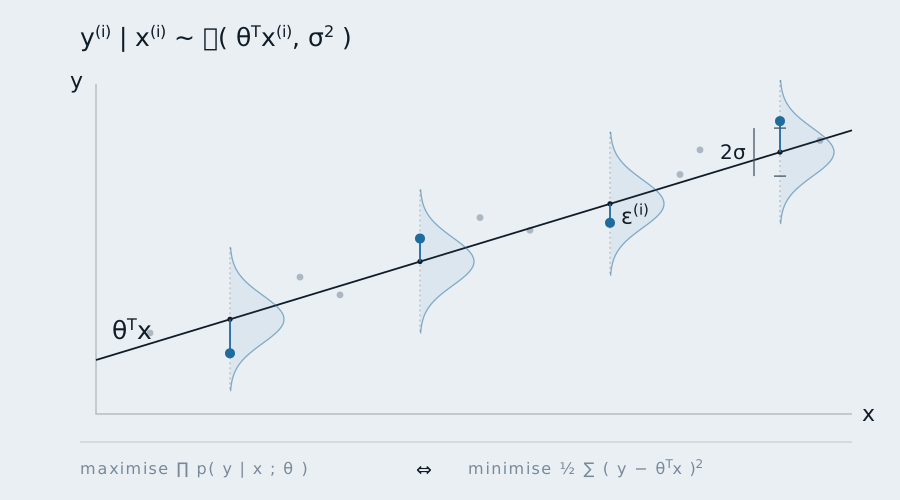
Each observation is drawn from a Gaussian centred on the regression line, so maximising the likelihood is the same as minimising the sum of squared residuals

Under this assumption, the distribution of y can be expressed as

P(y^{(i)}|x^{(i)};\theta) = \frac{1}{\sqrt{2\pi}\sigma} \text{exp}(\frac{-(y^{(i)} - \theta^Tx^{(i)})^2}{2\sigma^2})(5)

That indicates

y^{(i)} \sim \mathcal{N}(\theta^Tx^{(i)}, \sigma^2)(6)

The likelihood function

\begin{align} \mathcal{L}(\theta) &= P(\overrightarrow y|X; \theta) \\ &= \prod_{i=1}^{n} P(y^{(i)}|X^{(i)}; \theta) \\ &= \prod_{i=1}^{n} \frac{1}{\sqrt{2\pi}\sigma} \text{exp}(\frac{-(y^{(i)} - \theta^Tx^{(i)})^2}{2\sigma^2}) \end{align}(7)

The log likelihood function

\mathcal{l}(\theta) = n\log(\frac{1}{\sqrt{2\pi}\sigma}) + \sum_{i=1}^{n} \frac{-(y^{(i)} - \theta^Tx^{(i)})^2}{2\sigma^2}(8)

We can see here

l(\theta) \propto - \frac{1}{2} \sum_{i=1}^{n}(y^{(i)} - \theta^T x^{(i)})^2 = - \mathcal{J}(\theta)(9)

So we can see minimizing loss function \mathcal{J} is actually equivalent to find the maximum likelihood estimation of \overrightarrow y. This is the equivalence written along the bottom of the figure above: the squares are not an arbitrary choice of penalty, they are what a Gaussian error term turns into once you take a log.

References

machine learningloss functionprobability 大象無形