Tree-based methods contains a lot of tricks that are easily tested in data/machine learning related interviews, but very often mixed up. Go through these tricks while knowing the reasons behind could be very helpful in understanding + memorization.
Overview of Tree-based Methods
Overall speaking, simple decision/regression trees are for better interpretation (as they can be visualized), with some loss of performance (when compared to regression with regularization and non-linear regression methods, e.g. splines and generalized additive models). But with ideas including bagging, boosting and decorrelating, tree methods can be comparable with any other models in a lot of questions, but this, of course, reduce its interpretability.
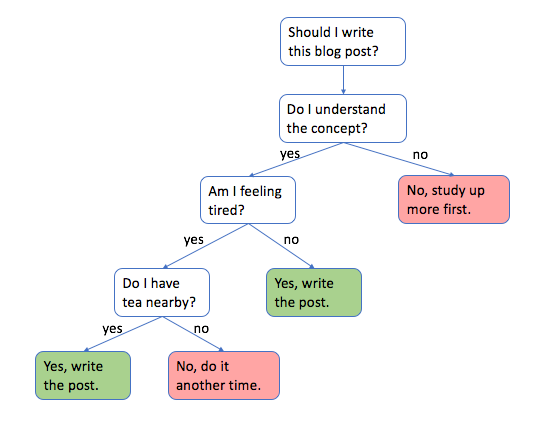
The idea of tree-based models is very simple – using different criteria to split training samples, so that in each bundle of separation, the samples are as “pure” as possible. This idea mimics the decision charts where we make two or more decisions for each question, and it finally leads to an outcome.
Below are 2 examples for decision tree in machine learning and decision tree in daily life respectively. The first figure is a case of binary classification, from the node to the leaves, the nodes are less and less “balance” (more “pure”). For the nodes in the final layer, Node 14, 13 and 22 contain just 1 class, which is considered good since the classification is perfect (on training set, this will be discussed later).

Growth of a Simple Tree
The growing algorithm is trying to achieve one thing: given a node with multiple samples inside, split them so that the resulting two nodes becomes as “pure” as possible. Here, “pure” means that for classification problem, the classes are less diverse; for regression problem, the dependent variable values in a single node should be as closed to each other as possible. For these two cases, there are respectively math representations to denote how “pure” the data is. Here are two examples:
Gini Index (classification problem):
$$G = \sum_{c=1}^{C}\pi_c(1 - \pi_c)$$
$\pi_c$ is the fraction of samples in the node that belongs to class $c$, and $C$ is all of the classes. Materials and references of Gini index is very abundant, so here I just want to make several side notes.
Gini index (or Gini impurity) is different from Gini coefficient in economics (which can also be called as Gini index, or Gini ratio)
Gini index in decision tree is similar (when taking $\log$) to a loss function in multi-class classification, cross-entropy loss:
$$L(\theta) = -\frac{1}{n}\sum_{i=1}^{n}\sum_{c=1}^{C}y_{ic}\log(p_{ic})$$
Residual Sum of Squares (RSS):
$$RSS = \sum_{i\in R_m}(y_i - \hat y_{R_m})^2$$
where $R_m$ a partition of tree (a node). And the prediction of a node $\hat y_{R_m}$ is determined by the average of values from all samples in the node.
1. Tree Pruning
Imaginably, if using the method described above for each node in the tree without limitation, finally one can easily get a perfect classification/regression tree (i.e. each node is “100% pure”). Even for the most difficult tasks, the tree can keep growing until there is only one data in each node, which is also a pure node.
But the problem for this is also obvious, the tree is too specific about the data, meaning that it’s over-fitting.
And to deal with this, some regularizations can be applied. And that includes specifying where the tree should stop growing. For example, it could be specifying:
- The maximum depth of the tree;
- The minimum number of samples in a node: e.g. stop splitting when there are only 10 samples in a node;
- etc… (can refer to
sklearn.tree.DecisionTreeClassifier)
Another thinking can be to add regularization weight after Gini/RSS loss in the growing algorithm. For example:
Cost complexity pruning, also known as weakest link pruning
$$\sum_{m=1}^{\mid T \mid}\sum_{}^{}(y_i - \hat y_{R_m})^2 + \alpha \mid T \mid$$
where $\alpha$ is a regularization hyperparameter and $\mid T \mid$ is the number of nodes in the tree. So this methods uses number of nodes to regularize the tree growing process.
Characteristics of Simple Decision/Classification Trees
- Very intuitive results and good interpretability with nice visualization.
- Intrinsic feature importance results. Presumably, if a feature is used closed to the root and divided a large amount of data, then the model considers the feature to be more important.
- There is a bias/variance trade-off. As described above, the more complex the tree is, the more flexible and better the tree would be in training set, but higher the risk of over-fitting.
- In most cases, simple tree performs worse than most other methods.
Other Tricks
So it comes to another topic: how to improve the performance of tree.
2. Bootstrapping aggregating (Bagging)
In most cases, tree’s can do well in training set but suffers in validation process. That is due to sometimes, a tree would accidentally think that one feature is important while that is actually an artifact in training set. To summarize, simple tree is too sensitive to data thus has high variance. For published models, it’s typical that an editor would ask the researches to include a sensitivity test for the models to ensure that the model is generalizable. This test is usually done based on the idea of bootstrapping.
So similarly here, if we want to make the tree to be more stable and less sensitive to data, we can consider the idea of bootstrapping, and that is adapted as bagging, which is also called bootstrapping aggregating.
The idea is pretty simple: bootstrap the training data, and build an independent tree based on each bootstrapped data. When predicting, use majority vote (classification) or average of predictions from all the trees built.

Out-of-Bag Error Estimation or OOB comes with the idea that for each tree, there are some samples are not included in bootstrapped samples (out of bag) thus can be used to evaluate the performance. The out-of-bag samples would averagely be $\frac{1}{3}$ of all data.
3. Limiting the number of predictors (Random Forest)
The idea of Random Forest (RF) is adding one more thing upon bagging: limiting the number of predictors. In doing so, random forest decorrelates the trees more. Typically, a tree is allow to randomly select $m$ features out of total $P$ features, where $m = \sqrt{P}$ or $m = \log_2{P}$ (refer to sklearn.ensemble).
4. Boosting
Boosting is another idea that share some common points with bagging but there are also differences. Similarly, boosting also seek to build multiple trees and use all of them to make predictions, and boosting is also very general idea that can be applied not only on tree methods but also some other ML methods as well.
Boosting is based on the idea of “fitting the residual”. It grows trees sequentially, and each tree is fitting the residual of current predictions and true values, in stead of fitting the response directly. To ensure generalizability, the model deliberately to let itself converge “slowly”, this is controlled by adding a parameter: shrinkage parameter $\lambda$. Typically selected between 0.01 and 0.001. Consider the bth tree to be a mapping of $\hat f^b$, and the total number of trees is $B$. Then, with the shrinkage parameter $lambda$, the prediction made by this boosting model can be expressed as:
$$\begin{align}\hat f(x) = \sum_{b = 1}^{B} \lambda \hat f^b(x)\end{align}$$