Thanks to nice illustrative pictures of LSTMs and RNNs by colah’s blog.
Recurrent neural networks (RNNs) use the same set of parameters to deal with inputs that are sequential. Inputs are usually broke into pars of same lengths, and fed into RNNs sequentially. In this way, the model learned and preserve the information from sequences of arbitrary lengths. This trait becomes very useful in natural language use cases where a model that is capable of dealing with sentence of any length is needed. Each set of parameters together, forms a RNN node/module/unit, however, some structures of RNN nodes have advantages over others.

LSTM
LSTM, or long Short-term memory, is a kind of structure of RNN node. It was originally developed by Sepp Hochreiter and Jürgen Schmidhuber in 1997 and improved by Gers et al. in 1999. The idea behind is that long term dependencies in other RNN units like GRU is hard to preserve and thus limits the ability to process longer sequence (e.g. long sentences). Thus LSTM comes up with two “hidden states”, one more short-term oriented (hidden state), another for “long-term” memory (cell state), to enable the model to link information in long distance. The two figures below showed a comparison between standard RNN and LSTM module.


Directly from the overview of the graph, we can see that LSTM provides more detailed interactions of parameters and hidden states inside each node, and then eventually achieved better performance by have both long-term and short-term memories preserved. We will go through the details of each step inside and be very clear about what is going on in a LSTM module.
Step-by-Step LSTM Walk Through
This section is heavily inspired by colah’s blog’s post.
Inputs and Outputs
Before going to the most details of operations happening in LSTM, let’s summarize what goes inside and outside a LSTM.
Inputs:
- $X_t$, Model input at time point $t$. Blue circles in the figure, remember RNNs and process sequential information of any length, so every RNN can take a input at each time point. In NLP, this $X_t$ is usually a word embedding vector of length $l$.
- $h_{t-1}$, hidden state from previous time point. Showed in the figure by the lower horizontal black line. This hidden states goes through each iteration of LSTM computation. And served as a symbol of short-term memory in LSTM. we will find out why real quick.
- $c_{t-1}$, cell state from previous time point. Showed in the figure by the upper horizontal black line. Very similar to hidden states in that it also passes through each iteration. But, it’s long-term memory.
Outputs:
- $h_t$, hidden state at this time point. Note that hidden states is also model output of each time step. (e.g. in language models, the model outputs a prediction of the next word, if using LSTM, then the word embedding was computed from hidden state of LSTM)
- $c_t$, cell state at this time point.
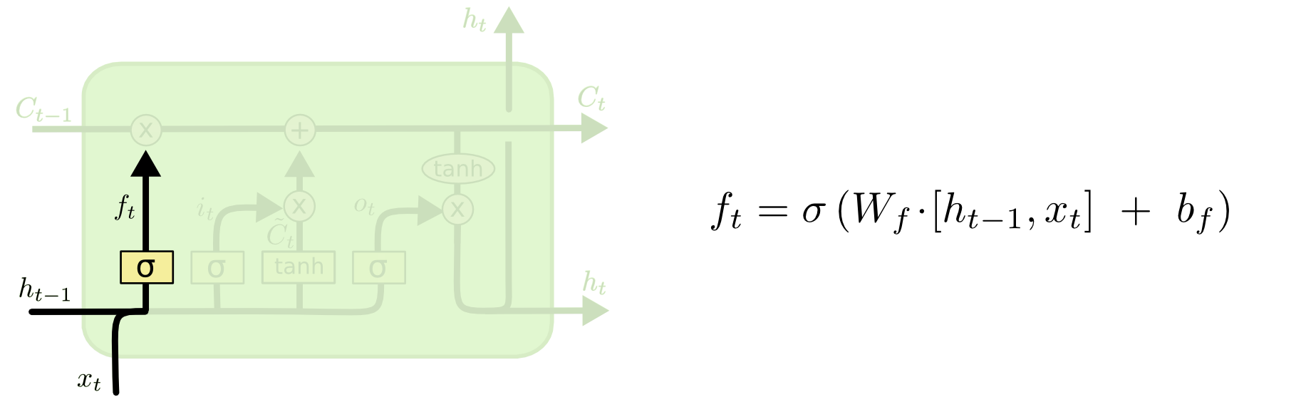
Step 1: Forget Gate
The first step of LSTM calculation is to decide, at this time point, should we choose to forget those memories or still keep them. And that decision was made by the operation of “forget gate”. The way that forget gate decide whether to forget, is by applying its knowledge (stored as two parameter matrices $$W_f$$ and $$b_f$$) to “examine” the previous hidden state ($h_{t-1}$) and new input ($x_t$). Sigmoid function is applied to round the result between 0 and 1, a $1$ represents “completely keep this” while a $0$ represents “completely forget this".
I think it makes most of sense when we think of the cell state as some memory that can be passed from long time ago, and hidden state is some new memory. Something new struck the “brain” of LSTM to let it forget the ancient memories. Keep this analog in mind in all later steps and you will find them more understandable.
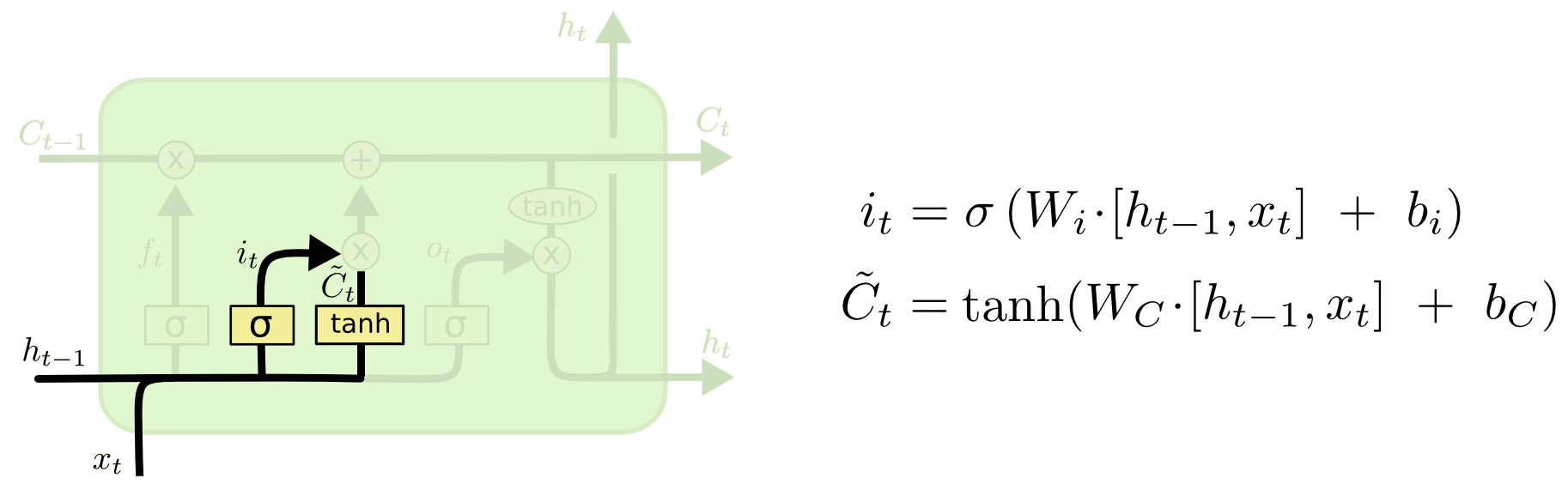
Step 2: Input Gate
Input gate decides what new information to write in the long-term memories. It performs exactly the same operation as forget gate to compute the value of input gate, ranging from 0 to 1, deciding none or all of the information should be written in the cell-state. The new cell state information is computed also by the previous hidden state ($h_{t-1}$) and new input ($x_t$), with a new activation function tanh (it implies that new cell state would be between -1 and 1).
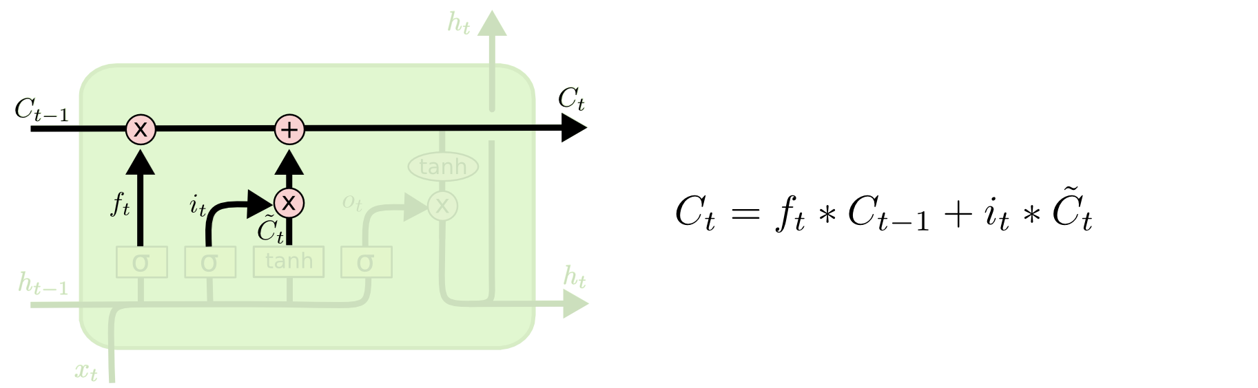
Step 3: Compute Cell State
Then, the new cell state is computed by adding what’s remaining after forget gate and what’s new computed by input gate.
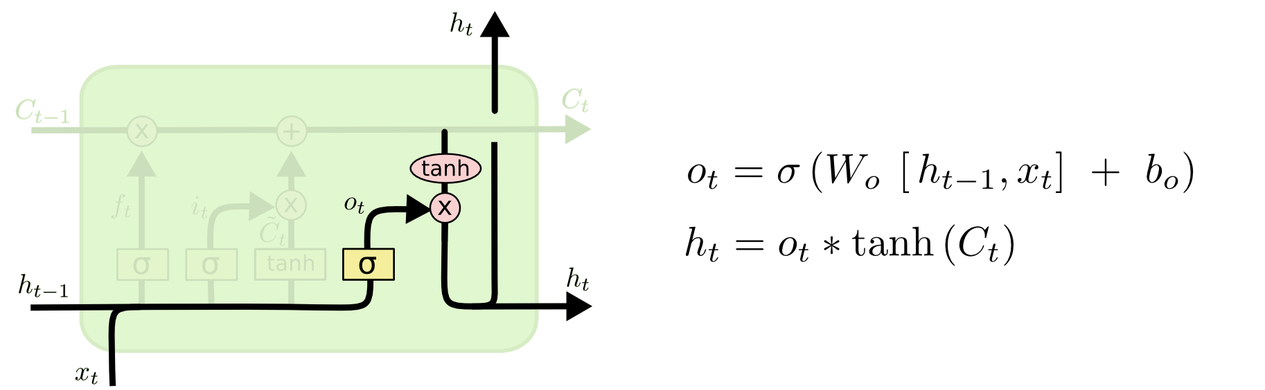
Step 4: Output/Hidden State, Output Gate
Similarly, the previous hidden state concatenated with input $x_t$ together decides what information to output by computing a output gate using sigmoid function. And then, the updated cell state though a tanh function, computes the new hidden state, thus the output of this module.
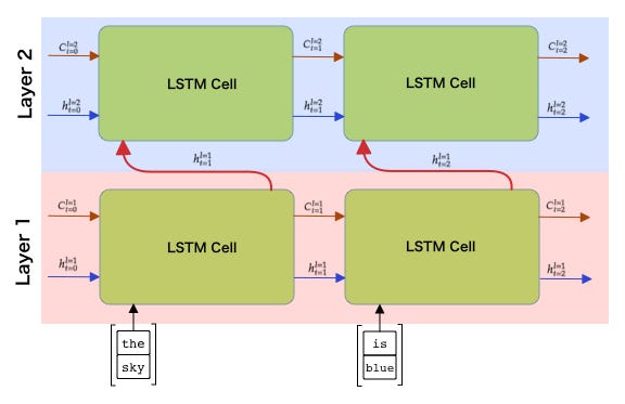
Multilayer LSTM
In some cases including language modeling, using multi-layer LSTM with similar amount of parameter would outperform single layer LSTM. In most cases, 2-layer LSTM would have a dramatic increase in performance comparing to 1-layer, and 3-layer would have a fraction of increase.
References
[1]: Hochreiter, Sepp, and Jürgen Schmidhuber. “Long short-term memory.” Neural computation 9.8 (1997): 1735-1780.
[2]: Gers, Felix A., Jürgen Schmidhuber, and Fred Cummins. “Learning to forget: Continual prediction with LSTM.” (1999): 850-855.
[3]: Understanding LSTM Networks – colah’s blog
[4]: Stanford CS 224N | Natural Language Processing with Deep Learning