EM And GMM
Expectation-maximization(EM) algorithm, provides a way to do MLE or MAE when there is incomplete data or unobserved latent variables.
NOTE: EM is general way of getting MLE or MAE estimations, not necessarily for clustering.
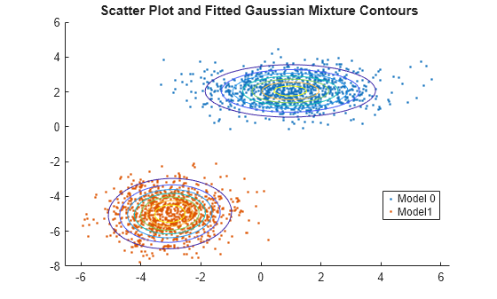
Gaussian mixture model(GMM) is a statistical model that can serve as a clustering algorithm. It assumes the data points to be from several gaussian distributions and uses EM algorithm to obtain the MLE estimations of those gaussians.(See plot)
Started from GMM algorithm.
GMM Algorithm
Description of the Model
Remember in K-means algorithm, which is also a cluster algorithm, it assigned each data point to a cluster by calculating the distance between the point and the cluster centroids and assigned to the closest one (See gif). Fitting a K-means algorithm consists of iteratively :
- Assign each point to a cluster;
- Update the centroid of each cluster.

Image GMM algorithm is trying to do a similar thing, with some modifications:
- Assume each cluster is sampled from a gaussian distribution;
- And there is a probability for a data point to be sampled from certain cluster;
So, it is almost like a parametric method of K-means algorithm. And fitting a GMM consists of (very roughly):
- Estimate the probabilities of each point being in each cluster (gaussian);
- Update the parameters of each cluster (mean and variance of gaussian).
Mathematical Definition
Model Setting
NOTE: $x^{(i)}$: data points ;$K$: number of clusters (pre-determined just like k-means); $z^{(i)}=j$: latent variable, means “Data point $x^{(i)}$ comes from cluster $j$”;
Given: $x^{(1)}, x^{(2)}, \dots, x^{(n)} \in \mathbb{R}^d$ and $K \in \{1,2,3,\dots\}$.
Do: find $z^{(i)}=j$’s probability $p(z^{(i)}=j)$: the probability that a point $x^{(i)}$ is sampled from cluster $j$.
Model: $$ p(x^{(i)}, z^{(i)}=j) = p(x^{(i)}| z^{(i)=j})p(z^{(i)}=j) \\ z^{(i)} \sim \text{Multinomial}(\phi) \\ x^{(i)}| z^{(i)}=j \sim N(\mu_j, \sigma^2_j) $$ By words, the model assumes:
- The probability of $z^{(i)}|x^{(i)}$ can be obtained by joint distribution of $x^{(i)}, z^{(i)}$, which is given by two “simpler” form of distributions that we can estimate;
- Latent variable $z^{(i)}$ is Multinomial;
- $x^{(i)}$ given $z^{(i)}$ is Gaussian.
Model Fit
Fitting the model requires the EM algorithm.
The EM Algorithm
The EM algorithm consists of iterating two steps, which very much resemble the two steps in k-means algorithm. The differences between EM and directly MLE is that EM algorithm, which is dealing with missing data or latent variables, adds a step (E-step) to estimate them, and uses its estimation to do MLE (M-step).
Description of the Idea
Assume that the distributions of $z^{(i)}$ and $x^{(i)}|z^{(i)}$ are parametrized by $\theta$. Then, ultimately, we want to find $\theta$ such that: $$ \begin{align} \theta_{MLE} &= arg\max_{\theta}l(\theta) \\ &= arg\max_{\theta}\sum_{i=1}^{n}\log p(x^{(i)};\theta) \end{align} $$ But we cannot optimize that directly. Here are some observations:
- Most obviously, we do not know the pdf of $x$.
- We can write $p(x^{(i)};\theta) = \sum_{j=1}^{K} p(x^{(i)}| z^{(i)}=j;\theta)p(z^{(i)}=j;\theta)$, which we made assumptions on, can we estimate using these? While for Gaussian distribution, we can estimate its parameters using MLE by calculating the gradients, it is not feasible to directly done here as the gradient depends on $p(z^{(i)}=j;\theta)$, which were not observed, and also requires estimation;
- On the other hand, the gradients regarding the Multinomial distributions depends on Gaussians;
- So, a simple way of optimizing the log-likelihood other than directly calculating gradient is needed.
The main idea, which was hinted in the observations, is that we have an annoying structure that makes the calculation to be very complicated $$ \log \sum_{j=1}^K(p(x^{(i)}| z^{(i)}=j;\theta)p(z^{(i)}=j;\theta)) $$ So directly maximizing $l(\theta)$ is not a good idea.
THOUGHT 1 (goal): Find a function $f(\theta)$, such that $$ arg\max_{\theta}l(\theta) = arg\max_{\theta}\sum_{i=1}^{n}f_{x^{(i)}}(\theta) $$ and $f(\theta)$ has a nicer form to estimate by taking gradients.
THOUGHT 2 (failed try): Recall Jensen’s inequality, we have $$ \begin{align} \log &\sum_{j=1}^K(p(x^{(i)}| z^{(i)}=j;\theta)p(z^{(i)}=j;\theta)) \\ &= \log \sum_{j=1}^Kp(x^{(i)}, z^{(i)};\theta)\\ &\geq \sum_{j=1}^K\log(p(x^{(i)}, z^{(i)};\theta)) \end{align} $$
If $$f_{x^{(i)}}(\theta) = \sum_{j=1}^K\log(p(x^{(i)}, z^{(i)};\theta))$$, the summation is out of the way, and $$p(x^{(i)}, z^{(i)})$$ can be easily expressed by the model.
NOT WORKING!: Though $p(x,z)$ has a nice form, maximizing the latter does not guarantee maximizing the previous!.
THOUGHT 3 (brilliant): Let $f(\theta)$ to be $$ f_{x^{(i)}}(\theta) = \sum_{j=1}^{K}Q_j\log \frac{p(x^{(i)}, z^{(i)}; \theta)}{Q_j} $$ where for $\forall j \in {1,\dots, K}, Q_j > 0$ and $\sum_j Q_j = 1 $. Some observations:
- Easy to see, we are also using $p(x, z)$ here, so easily estimated checked;
- “Mysterious” variable $Q_j$s are introduced, which satisfies some conditions. Those conditions make $Q_j$ to be able to serves as the pdf function of a discrete R.V.;
- Most importantly, we can show: maximizing $f$ is related to maximizing $l$:
$$ \text{Suppose } \theta_M = arg\max_{\theta}f(\theta) \\ \begin{align} f(\theta_M) - f(\theta) &= \log(p(x^{(i)};\theta_M)) - \log(p(x^{(i)};\theta)) - \sum_{j=1}^{K}Q_j \log \frac{p(z^{(i)}|x^{(i)};\theta)}{p(z^{(i)}|x^{(i)};\theta_M)} \\ \log(p(x^{(i)};\theta_M)) - \log(p(x^{(i)};\theta)) &= f(\theta_M) - f(\theta) + \sum_{j=1}^{K}Q_j \log \frac{p(z^{(i)}|x^{(i)};\theta)}{p(z^{(i)}|x^{(i)};\theta_M)} \end{align} $$
These means:
- We maximized $f(\theta)$ by taking $\theta_M$;
- log-likelihood $l(\theta)$ will be increasing (at least not decreasing) if $\sum_{j=1}^{K}Q_j \log \frac{p(z^{(i)}|x^{(i)};\theta)}{p(z^{(i)}|x^{(i)};\theta_M)} > 0$
- $\sum_{j=1}^{K}Q_j \log \frac{p(z^{(i)}|x^{(i)};\theta)}{p(z^{(i)}|x^{(i)};\theta_M)} > 0$ is obtained if we let
$$ Q_j = p(z^{(i)}|x^{(i)};\theta) $$
Wrap up the Idea
- Do not try to obtained $\theta_{MLE}$ by maximizing
$$ l(\theta) = \sum_{i=1}^{n}\log p(x^{(i)};\theta) $$
- Introducing $Q(z^{(i)}) = p(z^{(i)}|x^{(i)};\theta)$, and maximizing $f(\theta)$
$$ f(\theta) = \sum_{j=1}^{K} Q(z^{(i)})\log \frac{p(x^{(i)}, z^{(i)}; \theta)}{Q(z^{(i)})} $$
NOTE: $f(\theta)$ is actually an expectation $f(\theta) = E(log\frac{p(x^{(i)}, z^{(i)}; \theta)}{Q(z^{(i)})} | x^{(i)}; \theta)$
Naturally, we can see how this idea works: First, re-estimate $Q(z^{(i)})$ according to new $\theta$. Then, update $\theta$ with renewed $Q(z^{(i)})$. Let’s properly write down this idea.
##Formalizing the Algorithm
- E-STEP: GIVEN = {$X$, $\theta$}; DO = calculate
$$ Q_j(z^{(i)}) := p(z^{(i)}=j|x^{(i)};\theta) $$
- M-STEP: GIVEN = $Q_j(z^{(i)})$; DO = estimate parameters $\theta$
$$ \theta := arg\max_{\theta}\sum_{i=1}^{N}\sum_{j = 1}^{K}Q_j(z^{(i)})\log \frac{p(x^{(i)}, z^{(i)}; \theta)}{Q_j(z^{(i)})} $$
GMM Cheat sheet
- E-STEP:
$$ \begin{align} Q_j(z^{(i)}) :&= \frac{p(x^{(i)},z^{(i)=j};\theta)}{p(x^{(i)})} \\ &= \frac{p(x^{(i)}|z^{(i)=j};\theta) p(z^{(i)}=j)}{\sum_{j=1}^{K}p(x^{(i)}|z^{(i)};\theta) p(z^{(i)}=j)} \end{align} \\ $$
- M-STEP:
$$
\begin{align}
\phi_j :&= \frac{1}{n} \sum_{i=1}^{n}Q_j(z^{(i)}) \\
\mu_j :&=\frac{\sum_{i=1}^{n}Q_j(z^{(i)})x^{(i)}}{\sum_{i=1}^{n}Q_j(z^{(i)})} \\
\Sigma_j :&= \frac{\sum_{i=1}^{n}Q_j(z^{(i)})(x^{(i)} - \mu_j)(x^{(i)} - \mu_j)^T}{\sum_{i=1}^{n}Q_j(z^{(i)})}
\end{align}
$$